






Phase space generators#
Amplitude analysis needs samples of four-momenta that are distributed uniformly over the phase space of a decay. TFPhaseSpaceGenerator produces such samples with phasespace. That package generates weighted events, so TFPhaseSpaceGenerator turns them into unweighted events with a hit-and-miss step: an event is kept if a uniform random number is below its weight. This page shows how the adaptive_max_weight option makes that step faster without changing the generated distribution.
Hit-and-miss against an estimated maximum weight#
By default, the random numbers of the hit-and-miss step are drawn up to \(1\), the upper bound of the normalized weights that phasespace guarantees. The weights that actually occur are often far below that bound, especially for decays into many particles, so most events are rejected. With adaptive_max_weight=True, the random numbers are drawn up to an estimate of the maximum weight instead. The estimate is the largest weight seen so far plus a margin of 5%. If a later bunch contains a larger weight, the estimate is raised and the sample is generated anew, so that the result remains unbiased.
The option is keyword-only and is off by default, so existing code keeps producing the same events for the same seed.
The following plots illustrate this for a \(5\,\mathrm{GeV}\) particle that decays into an increasing number of pions. The left panel shows the weight distributions relative to the largest weight in each sample. The right panel shows the fraction of events that survive the hit-and-miss step: with the default setting, this is the mean weight, while with adaptive_max_weight=True it is the mean weight divided by the estimated maximum.
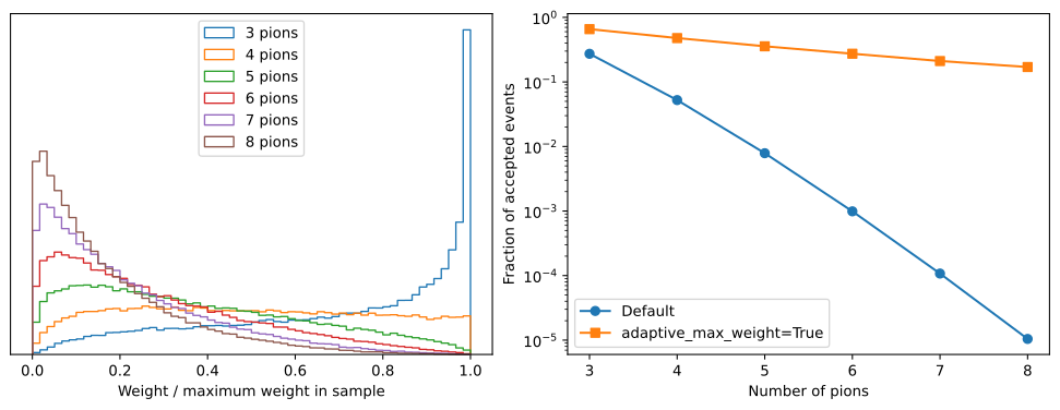
The shape of the weight distribution relative to its maximum changes only moderately with more particles, but the mean weight relative to the bound of \(1\) drops by several orders of magnitude. With the estimated maximum, the fraction of accepted events stays above 10%. The gain in speed grows accordingly: for five or more pions, generation is orders of magnitude faster. TR-038 benchmarks this and confirms with statistical tests that both settings produce the same distributions.
Usage#
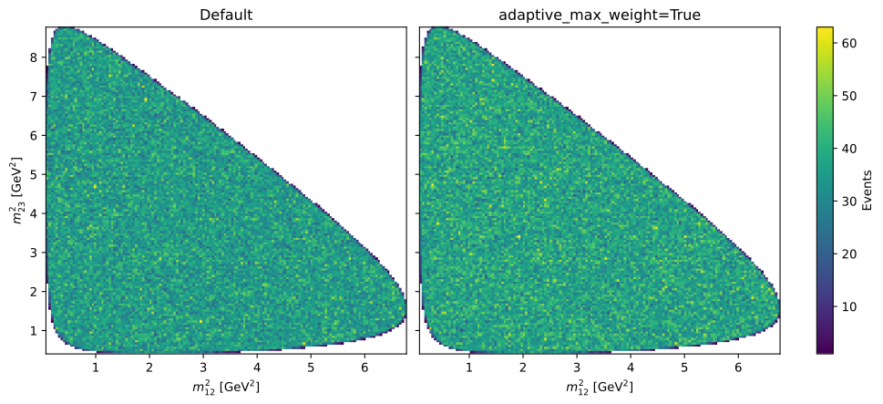
The option is a keyword argument of TFPhaseSpaceGenerator. The following example generates a sample of a three-body decay with both settings. The events differ, because the hit-and-miss step consumes the random numbers differently, but both samples are distributed uniformly over phase space: the events fill the kinematically allowed region of the Dalitz plot evenly.
from tensorwaves.data import TFPhaseSpaceGenerator, TFUniformRealNumberGenerator

initial_state_mass = 3.0969
final_state_masses = {0: 0.1350, 1: 0.1396, 2: 0.4937}
default_generator = TFPhaseSpaceGenerator(initial_state_mass, final_state_masses)
adaptive_generator = TFPhaseSpaceGenerator(
    initial_state_mass, final_state_masses, adaptive_max_weight=True
)
size = 500_000
default_generator.show_progress = False
adaptive_generator.show_progress = False
samples = {
    "Default": default_generator.generate(size, TFUniformRealNumberGenerator(seed=0)),
    "adaptive_max_weight=True": adaptive_generator.generate(
        size, TFUniformRealNumberGenerator(seed=0)
    ),
}
When to use the option#
The option pays off for decays into five or more particles, where the default setting rejects most events. Keep the default when samples have to be identical to those of earlier versions for the same seed, for instance when tests compare against stored values. A small bunch_size makes the estimate of the maximum weight less accurate and leads to more restarts, so the option works best with the default bunch size.